Permafrost Modelling in the Himalaya: Three Days at ICIMOD

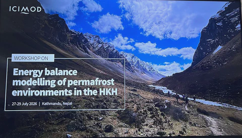 Workshop on Energy Balance Modelling of Permafrost Environments in the HKH, ICIMOD, Kathmandu. © 2026 ICIMOD
Permafrost underlies roughly one million square kilometres of the Hindu Kush Himalaya (HKH) i.e., about 14 times the area covered by the region’s glaciers, and more than the glacier area in nearly every HKH country (Gruber et al., 2017).
Almost none of it is monitored.
That asymmetry is the whole problem. Glaciers are visible from space, and we have decades of mass-balance records for them. Permafrost is invisible by definition: it is a thermal condition of the ground, not a landform. You cannot see it, and confirming it at a single site requires drilling a borehole and instrumenting it for years. Across the HKH, in-situ observations remain rare enough that most of what we know about where permafrost is, and how much of it there is, comes from models rather than measurements.
That has consequences beyond an academic data gap. Thawing permafrost destabilises rock slopes and moraines, undermines roads and buildings, and changes the timing of water release from high catchments. These are the kinds of processes that inform hazard assessment and infrastructure planning — and at present the region is largely planning without them.
Since the observations are unlikely to arrive at the scale required any time soon, physically-based models are the practical way forward. The obstacle is that few researchers in the region have been able to use them. That is what this workshop set out to change. Over three days at ICIMOD in Kathmandu, from 27 to 29 July, researchers, most of whom had never before compiled a hydrological model progressed to running and interpreting their own permafrost simulations.
Why a model, and not just more measurements
Permafrost is defined by temperature, not by ice content: ground that remains at or below 0 °C for two or more consecutive years. That distinction matters particularly in the cold-arid trans-Himalaya, where much of the frozen ground is coarse and dry — permafrost with very little ice in it is still permafrost. More boreholes would obviously help, and the region needs them. But three things limit what drilling alone can deliver.
Boreholes are points. Ground temperature in mountains varies over metres, not kilometres, because it depends on slope, aspect, snow accumulation and soil properties. In our own work in the upper Ganglass catchment in Ladakh, modelled active-layer thickness ranged from about 0.1 m to over 4 m within a single catchment (Wani et al., 2020). Interpolating between sparse boreholes across terrain like that is not a credible strategy.
Boreholes only describe the present. No measurement tells you what the active layer will do under 2 °C of warming. Only a process model can be asked that question.
The ground is slow. Permafrost responds to climate over years to centuries. A record of a few seasons cannot separate a genuine trend from ordinary variability, whereas a model can be run over the relevant timescales.
So the sensible strategy is not measurement or modelling, but measurement for modelling: enough observation to constrain and evaluate a physically-based model, then the model to extend those few points across space and time.
That, in turn, requires people who can run the models. And the barrier there is rarely the science but compilation errors, configuration files, and not knowing whether the number on the screen means anything.
How the three days were structured
Day 1: concepts, no computers. We deliberately spent the first day without touching a keyboard. Permafrost definitions and the ground thermal regime; what “numerical” actually means, from discretization through finite differences to initial conditions; and a full session on the surface energy balance, which is the engine driving everything below.
Day 2: the model. A two-hour introduction to GEOtop itself: its structure, the two coupled equations it solves, the multilayer snow scheme, and how terrain effects on radiation are handled. Then installation, and by the afternoon everyone had a point simulation configured and running.
Day 3: analysis and evaluation. Reading model output, plotting ground temperature profiles and active-layer behaviour, and comparing simulations against logger data. We finished with group projects.
What worked
Point simulations, not distributed ones. Every participant ran a single-column setup with all parameters inline: no DEM, no raster maps, no separate soil file. Three items in a folder: a configuration file, a meteorological forcing file, and an output directory. The physics is identical to a distributed run; only the input preparation grows. Starting simple meant nobody lost a day to file paths.
One-slide group projects. Every group started from the same working simulation and changed exactly one thing: removing snow, coarsening the soil layers, adding 2 °C to the air temperature, flipping the slope from north-facing to south. Each group wrote down what they expected before running, then presented one figure and one surprise.
Because each group changed something different, the closing discussion assembled into a picture no single group could have produced. Between them, they had done a sensitivity analysis of a permafrost model in an afternoon.
Course material
Everything is open-access under CC-NC BY 4.0:
| Material | Contents |
|---|---|
| Lecture slides | Conceptual foundations, surface energy balance, GEOtop model introduction |
| Hands-on guides | Installation, WSL setup for Windows, model configuration, first runs |
| Jupyter notebooks | Output analysis and model evaluation against observations |
| Sample case | A complete, runnable point simulation |
Links to be added — material is being uploaded.
Thanks
To ICIMOD for hosting and organising, to Raman Yadav (YIPP, ICIMOD) for co-instructing the hands-on sessions, and to the participants, who asked better questions than I was expecting on day one and considerably better ones by day three.
The postdoctoral work of JMW is supported by the SPACE IT UP project (ASI Contract n. 2024-5-E.0, CUP Master n. I53D24000060005).
Related resources
- GEOtop source code: github.com/geotopmodel/geotop
- GEOtop user manual: geotopmodel.github.io
- Previous course: Getting Started with GEOtop at EGU 2026
- Further reading: Permafrost Readings for Beginners
Key references:
- Gruber, S., Fleiner, R., Guegan, E., Panday, P., Schmid, M.-O., Stumm, D., Wester, P., Zhang, Y., Zhao, L. (2017). Review article: Inferring permafrost and permafrost thaw in the mountains of the Hindu Kush Himalaya region. The Cryosphere, 11, 81–99. DOI
- Endrizzi, S., Gruber, S., Dall’Amico, M., Rigon, R. (2014). GEOtop 2.0: simulating the combined energy and water balance at and below the land surface. Geosci. Model Dev., 7, 2831–2857. DOI
- Wani, J. M., Thayyen, R. J., Gruber, S., Ojha, C. S. P., Stumm, D. (2020). Single-year thermal regime and inferred permafrost occurrence in the upper Ganglass catchment of the cold-arid Himalaya, Ladakh, India. Sci. Total Environ., 703, 134631. DOI
- Wani, J. M., Thayyen, R. J., Ojha, C. S. P., Gruber, S. (2021). The surface energy balance in a cold and arid permafrost environment, Ladakh, Himalayas, India. The Cryosphere, 15, 2273–2293. DOI
If you are working on permafrost in the HKH, or thinking about instrumenting a site and wondering what a model would need from it, do get in touch.
